Top Guidelines Of Sumif Multiple Columns

If "blank" indicates cells that have definitely nothing - no formula, no zero size string returned by some other Excel function, after that utilize "=" as the standards, like in the complying with SUMIF formula: =SUMIF(A 2: A 10,"=", C 2: C 10) If "empty" includes no size strings (as an example, cells with a formula like =""), then make use of "" as the standards: =SUMIF(A 2: A 10,"", C 2: C 10) Both of the above formulas evaluate cells in column An as well as if any kind of vacant cells are discovered, the equivalent worths from column C are added.

Generally, you use the SUMIF feature to conditionally sum values based upon dates similarly as you use text and numerical criteria. If you intend to sum worths corresponding to the dates that are more than, much less than or equal to the date you specify, after that use the Standard Formula Instance Description Sum values based upon a specific day.

Sum values if a matching day is above or equivalent to an offered date. =SUMIF(B 2: B 9,">=10/29/2014", C 2: C 9) Sum values in cells C 2: C 9 if a matching day in column B is higher than or equal to 29-Oct-2014. Sum values if a corresponding date is above a day in an additional cell.

In instance you wish to sum worths based upon a present date, after that you have to use Excel SUMIF in combination with the TODAY() function as shown below: Standard Formula Instance Sum values based on the present day. =SUMIF(B 2: B 9, TODAY(), C 2: C 9) Amount values matching to a previous day, i.e.

Sumif Not Equal for Beginners

=SUMIF(B 2: B 9, "" & TODAY(), C 2: C 9) Sum values if a day occurs in a week( i.e. today +7 days).=SUMIF (B 2: B 9, "="& TODAY( )+7, C 2: C 9) The screenshot below illustrates just how you can utilize the last formula to discover the overall quantity of all items that deliver in a week. In Excel 2007 and also higher, you can additionally utilize the SUMIFS function that allows several criteria, which is also a much better alternative. While the last is the topic of our following short article, an example of the SUMIF formula complies with below: =SUMIF(B 2: B 9, ">=10/1/2014", C 2: C 9) - SUMIF(B 2: B 9, ">=11/1/2014", C 2: C 9) This formula summarize the worths in cells C 2: C 9 if a day in column B is between 1-Oct-2014 and also 31-Oct-2014, inclusive.

The very first SUMIF function builds up all the cells in C 2: C 9 where the matching cell in column B is higher than or equivalent to the start date (Oct-1 in this example). After that you simply need to deduct any values that fall after completion date (Oct-31), which are returned by the second SUMIF feature.

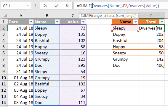
Suppose, you have a recap table of monthly sales. Since it was consolidated from a numbers of regional reposts, there are a few records for the very same item: So, exactly how do you locate the total amount of apples sold in all the states in the previous 3 months? As you remember, the dimensions of sum_range are identified by the dimensions of the array criterion.

This is not what we are seeking, right? The most rational and also easiest solution that recommends itself is to create an assistant column that determines individual sub-totals for each and every row and then referral that column in the sum_range standards. Go on and also position a simple AMOUNT formula in cell F 2, then load down column F: =AMOUNT(C 2: E 2) After that, you can compose a normal SUMIF formula similar to this: =SUMIF(A 2: A 9, "apples", F 2: F 9)or=SUMIF(A 2: A 9, H 1, F 2: F 9) In the above solutions, sum_range is exactly of the exact same size as array, i.e

Rumored Buzz on How To Use Sumif

. There can be a number of reasons Excel SUMIF is not helping you. In some cases, your formula does not return what you expect only since the data type in a cell or in some debate isn't suited for the SUMIF feature. So, below is a list of points to examine. The first (range) as well as third (sum_range) parameters of your SUMIF formula need to always be a variety reference like A 1: A 10.

Right formula: =SUMIF(A 1: A 3, "flower", C 1: C 3) Incorrect formula: =SUMIF( 1,2,3, "blossom", C 1: C 3) As nearly any kind of other Excel feature, SUMIF can reference other sheets and workbooks, provided they are presently open. For instance, the adhering to formula will certainly sum the worths in cells F 2: F 9 in Sheet 1 of Book 1 if a matching cell in column A if the very same sheet contains "apples": =SUMIF( [Schedule 1. xlsx] Sheet 1!$A$ 2:$A$ 9,"apples", [Book 1. xlsx] Sheet 1!$F$ 2:$F$ 9) Nevertheless, this formula will not work as quickly as Publication 1 is closed.

As noted at first of this tutorial, in contemporary versions of Microsoft Excel, the array and also sum_range specifications does not need to be equally sized. In Excel 2000 and also older, unequally sized range and also sum_range can trigger problems. Nevertheless, even in one of the most current variations of Excel 2010 as well as Excel 2016, complex SUMIF solutions where sum_range has much less rows and/or columns than array are picky.

If you've occupied your workbook with complicated SUMIF solutions that reduce down your Excel, look into The Excel SUMIF instances described in this tutorial just discuss several of the standard uses of this feature. In the next article, we'll investigate advanced formulas that harness the real power of SUMIF as well as SUMIFS and also allow you sum by numerous requirements.

An Unbiased View of Sumif Between Two Dates

I wish to do a sum of cells, with numerous criterias. I have discovered that the method to do it is with sumproduct. Similar to this =SUMPRODUCT((A 1: A 20="x")*(B 1: B 20="y")*(D 1:D 20)) The trouble I am having is that the A row includes joined cells (which I can not transform) In my situation I intend to do a sum of every number in the offered row under both 2010 and also 2011 conference my criterias.

excel sumif a color sumif excel formula sample excel sumif distinct